Quality control
During sequencing, the nucleotide bases in a DNA or RNA sample (library) are determined by the sequencer. For each fragment in the library, a short sequence is generated, also called a read, which is simply a succession of nucleotides.
Modern sequencing technologies can generate a massive number of sequence reads in a single experiment. However, no sequencing technology is perfect, and each instrument will generate different types and amount of errors, such as incorrect nucleotides being called. These wrongly called bases are due to the technical limitations of each sequencing platform.
Therefore, it is necessary to understand, identify and exclude error-types that may impact the interpretation of downstream analysis. Sequence quality control is therefore an essential first step in your analysis. Catching errors early saves time later on.
Assessing quality with FastQC
To take a look at sequence quality along all sequences, we can use FastQC. It provides a modular set of analyses which you can use to check whether your data has any problems of which you should be aware before doing any further analysis. We can use it, for example, to assess whether there are known adapters present in the data.
Installing FastQC
To install FastQC in Linux environment, we can use package management tool conda.
Terminal
$ conda install -c bioconda fastqc
Running FastQC
We can start FasQC program by typing fastqc into command line.
Terminal
$ fastqc
Now we can use File -> Open... and select a file we want to examine.
Per base sequence quality
With FastQC we can use the per base sequence quality plot to check the base quality of the reads.
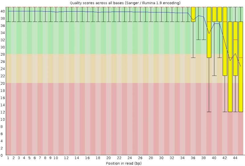
On the x-axis are the base position in the read. In this example, the sample contains reads that are up to 45 bp long. For each position, a boxplot is drawn with:
- the median value, represented by the central red line
- the inter-quartile range (25-75%), represented by the yellow box
- the 10% and 90% values in the upper and lower whiskers
- the mean quality, represented by the blue line
The y-axis shows the quality scores. The higher the score, the better the base call. The background of the graph divides the y-axis into very good quality scores (green), scores of reasonable quality (orange), and reads of poor quality (red).
Adapter Content
The plot shows the cumulative percentage of reads with the different adapter sequences at each position. Once an adapter sequence is seen in a read it is counted as being present right through to the end of the read so the percentage increases with the read length. FastQC can detect some adapters by default (e.g. Illumina, Nextera), for others we could provide a contaminants file as an input to the FastQC tool.
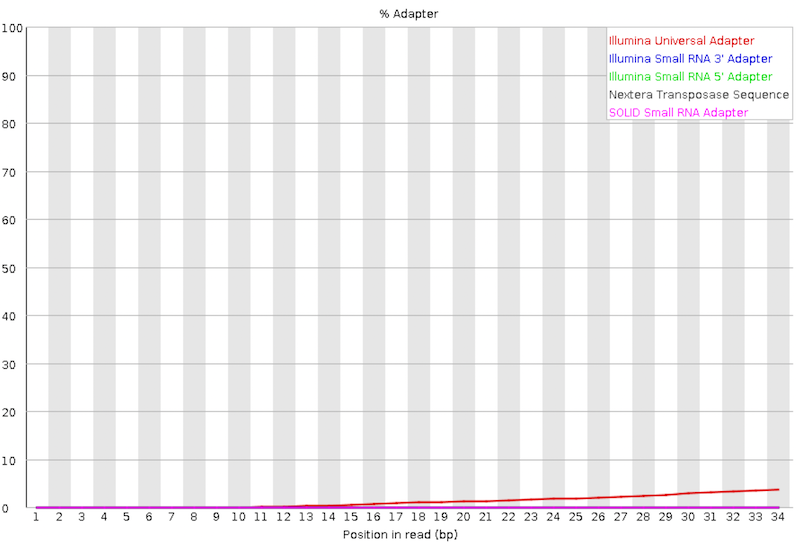
We can run an trimming tool such as Cutadapt to remove this adapter. We will explain that process in future section.
Per base sequence content
Per Base Sequence Content plots the percentage of each of the four nucleotides (T, C, A, G) at each position across all reads in the input sequence file. As for the per base sequence quality, the x-axis is non-uniform.
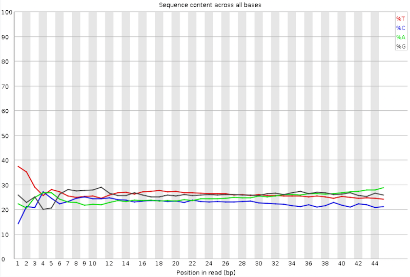
In a random library we would expect that there would be little to no difference between the four bases. The proportion of each of the four bases should remain relatively constant over the length of the read with %A=%T and %G=%C, and the lines in this plot should run parallel with each other. ChIP-seq data can encounter read start sequence biases in this plot if fragmenting with transposases.
Per sequence GC content
This plot displays the number of reads vs. percentage of bases G and C per read. It is compared to a theoretical distribution assuming an uniform GC content for all reads, expected for whole genome shotgun sequencing, where the central peak corresponds to the overall GC content of the underlying genome. Since the GC content of the genome is not known, the modal GC content is calculated from the observed data and used to build a reference distribution.
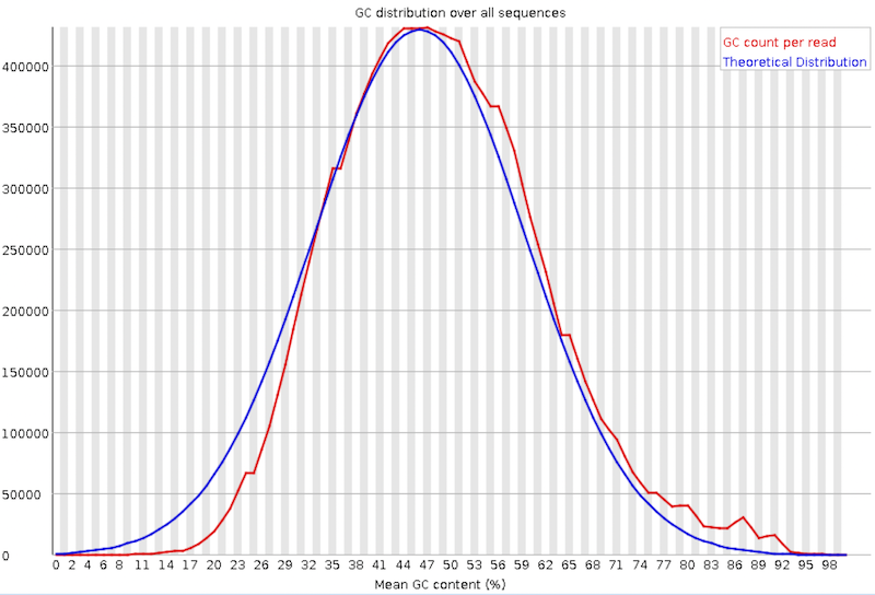
An unusually-shaped distribution could indicate a contaminated library or some other kind of biased subset. A shifted normal distribution indicates some systematic bias, which is independent of base position. If there is a systematic bias which creates a shifted normal distribution then this won’t be flagged as an error by the module since it doesn’t know what your genome’s GC content should be.
But there are also other situations in which an unusually-shaped distribution may occur. For example, with RNA sequencing there may be a greater or lesser distribution of mean GC content among transcripts causing the observed plot to be wider or narrower than an ideal normal distribution.
Sequence Duplication Levels
The graph shows in blue the percentage of reads of a given sequence in the file which are present a given number of times in the file.
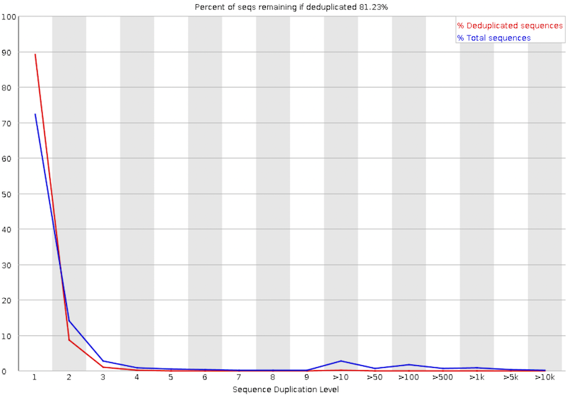
In a diverse library most sequences will occur only once in the final set. A low level of duplication may indicate a very high level of coverage of the target sequence, but a high level of duplication is more likely to indicate some kind of enrichment bias.
Two sources of duplicate reads can be found:
- PCR duplication in which library fragments have been over-represented due to biased PCR enrichment. It is a concern because PCR duplicates misrepresent the true proportion of sequences in the input.
- Truly over-represented sequences such as very abundant transcripts in an RNA-Seq library or in amplicon data (like in our sample). It is an expected case and not of concern because it does faithfully represent the input.
| Previous page | Home | Next page |